Interactive Time Series Analysis Tool

Motivation

An interactive time series analysis toolkit for exploring, forecasting, and evaluating real-world data. This tool is intended for analysts and data scientists exploring time series data and evaluating forecasting approaches.

This tool allows users to rapidly compare forecasting methods, test model performance on historical data and quantify forecast accuracy — all without rerunning complex pipelines. Designed for flexibility and transparency, it supports common workflows such as resampling, filtering, and model selection across a range of time series problems.

Local data files can be used or the latest exchange rates of major currencies.

The project emphasises practical forecasting: not just generating forecasts, but understanding how reliable they are in real-world scenarios.

The focus is not just on generating forecasts, but on understanding when they can be trusted.

Usage

Run the notebook and follow the interactive prompts to:

1. Load data

2. Select variables

3. Choose model and forecast horizon

4. Evaluate forecasts

These steps can be adjusted interactively without needing to rerun the entire pipeline.

Supported Methods

• Exponential Smoothing
• Holt-Winters (Triple Exponential)
• Auto-ARIMA
• Prophet (with holiday effects)

Additional methods can be incorporated as needed.

Why this tool?

• Quickly compare forecasting methods without rebuilding pipelines
• Evaluate model performance using backtesting
• Quantify prediction error in interpretable terms
• Explore real-world datasets interactively

Key Insight

In practice, forecasting models often appear accurate in-sample but fail in real-world conditions. This tool highlights that gap through built-in backtesting and error analysis.

Forecast accuracy depends heavily on market conditions. Even well-performing models may fail to predict sudden structural changes, as demonstrated in the stock price example.

Requirements

pandas
numpy
matplotlib
statsmodels
prophet
ipywidgets
yfinance

Note

By default the notebook (TS.ipynb) will run a demo using AirPassengers.csv with limited interactivity. To run with full interactivity change

 USE_DEFAULTS = True
 to
 USE_DEFAULTS = False

at the bottom of the first cell.

Example 1

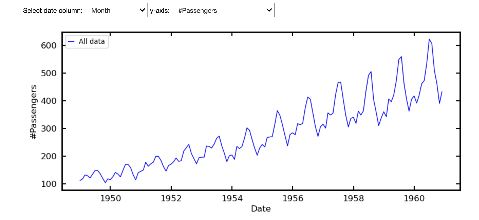
For a simple example, which requires no filtering, we follow Exponential Smoothing for Time Series Forecasting which works from the AirPassengers.csv dataset. We selected this via the Local CSV option (Currency Rates are also available).

The plot will be displayed, as well as the option to select the axes when there are choices available.

There is then the option to filter the data, which is not necessary here but see Example 2.

You can then:

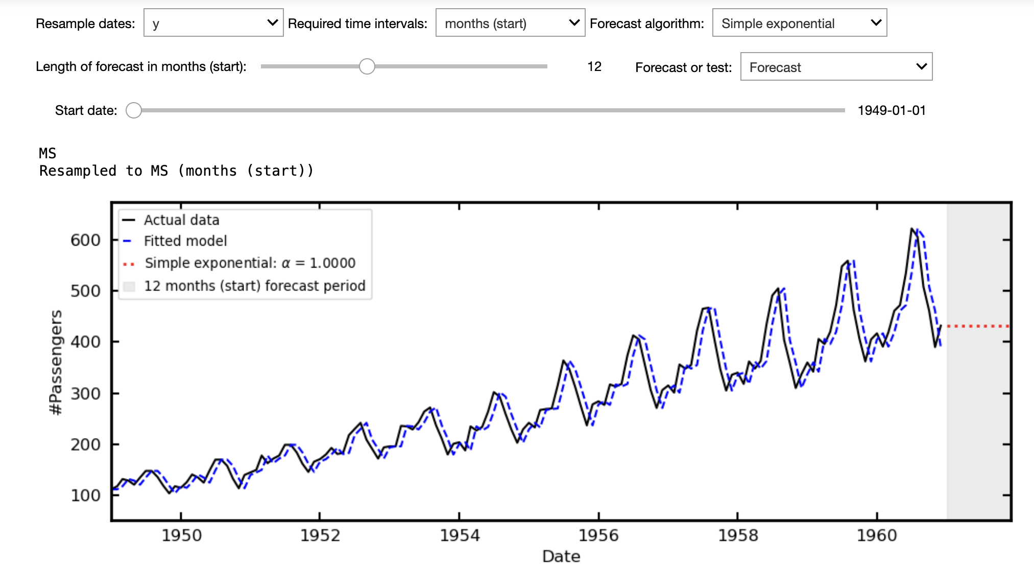
• Resample the data, e.g. from days to business days (this will generally remove any "no frequency information" warning).
• Choose the forecast algorithm - Prophet includes the options to model holidays for some countries
• Select the length of the forecast
• Have the option to test the forecast from historical data. This reserves the most recent data, according to the forecast length, to be compared directly with the predicted values. That is, how well the model performs on unseen data
  • The result is quantified via the Root Mean Square Error, RMSE = $\sqrt{\frac{1}{n}\sum_{i=1}^n(\hat{y} - y_i)^2}$.
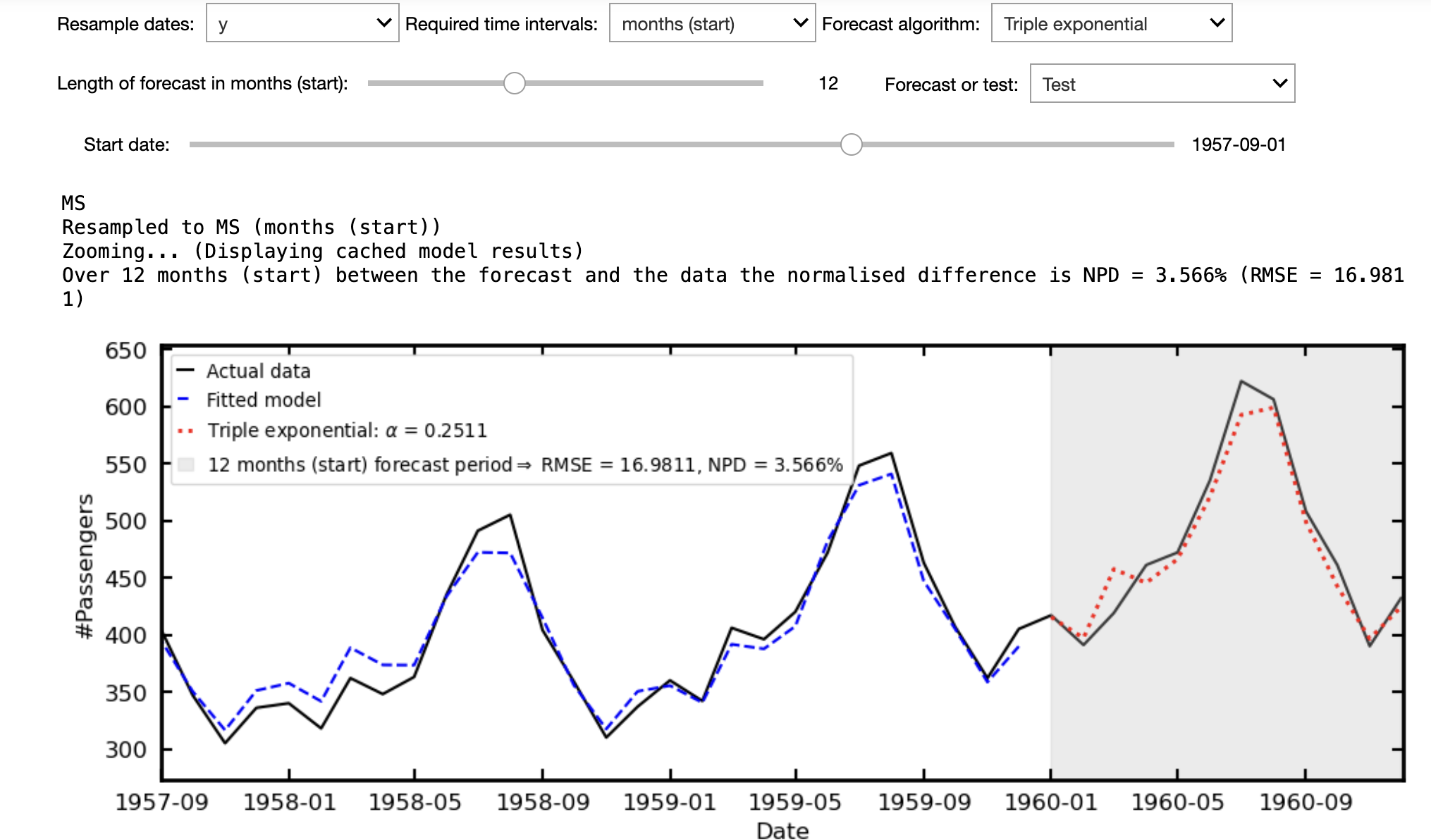
• The normalised percentage difference, which scales the RMSE over the mean value of the observed data over the forecast period, NPD $\equiv 100\times{\rm RMSE}/\mu_{\rm actual}$.
• Zoom in on the forecast range for closer inspection

E.g. in the following, where the triple exponential method has been used to make 12 month forecast we can compare this with how the data actually evolved over this period. This offers the option of saying "well the forecast was pretty accurate, just 3.6% out, maybe I can trust it to forecast the next 12 months".

Example 2

The historical stock price data, all_stocks_5yr.csv, used by Master Simple Exponential Smoothing for Time Series Forecasting does require filtering. I have merged this with another dataset into all_stocks_5yr+names.csv, where the Security field has the registered name of the company.

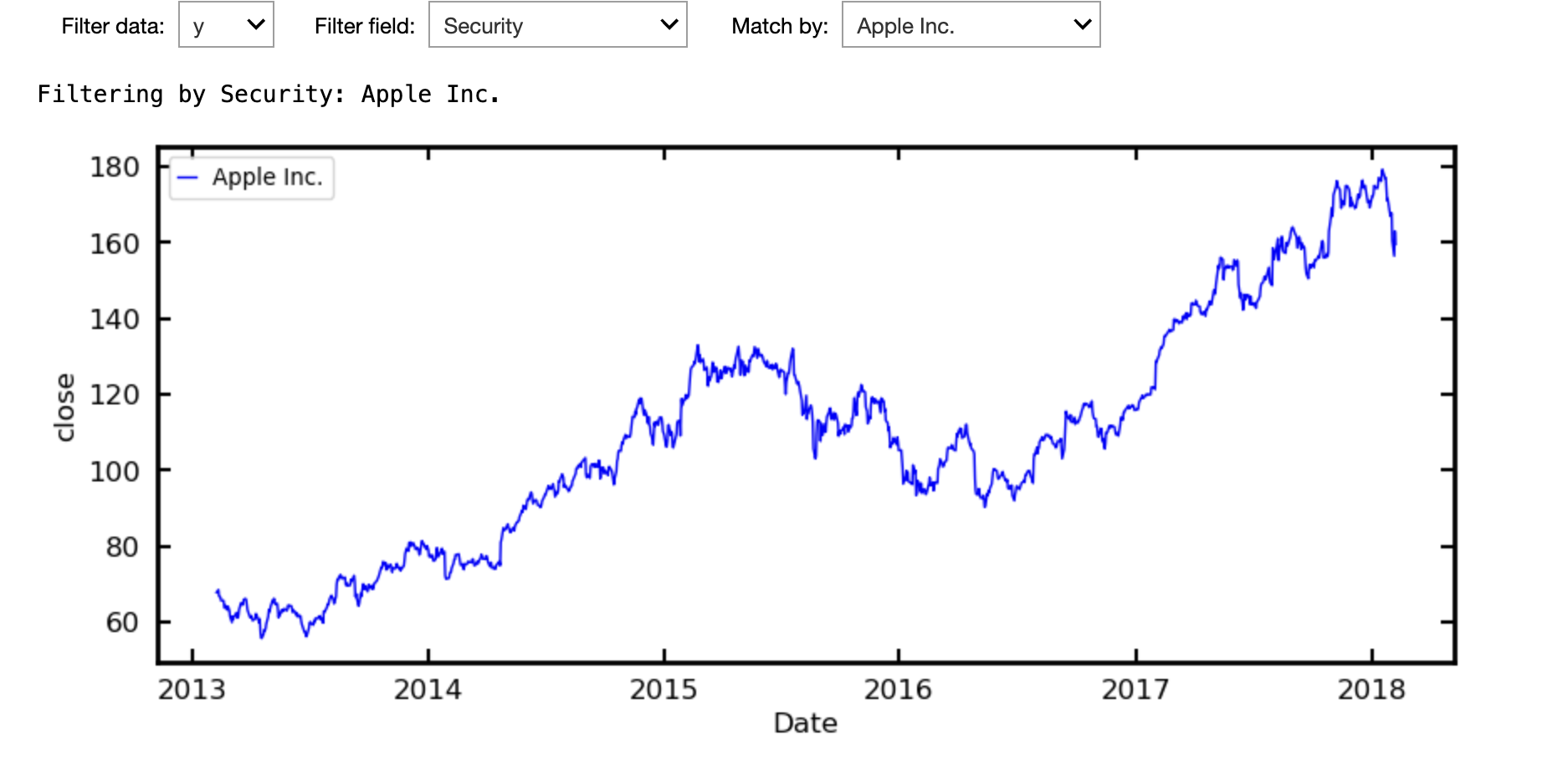
Following their example, we can plot the closing price against the date, but obtain the following.

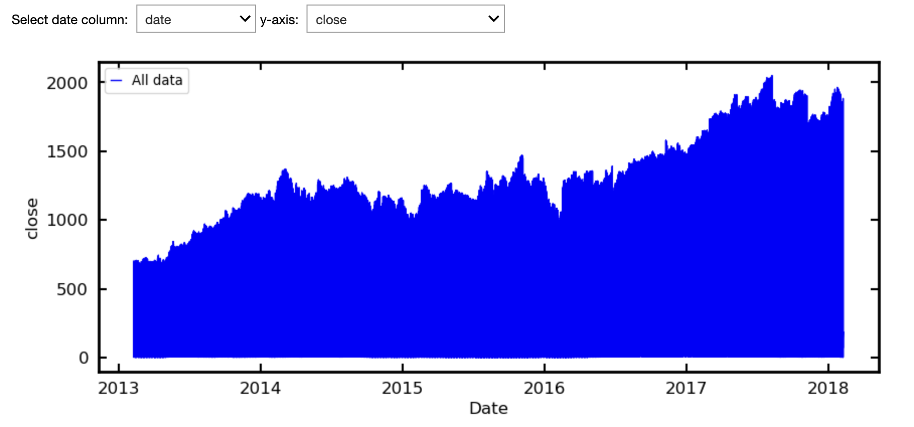
This is because the closing prices for all 505 companies are shown. We can use the drag down menu to select the name of the company we want.

Resampling from days to business days, auto ARIMA gives the forecast below.

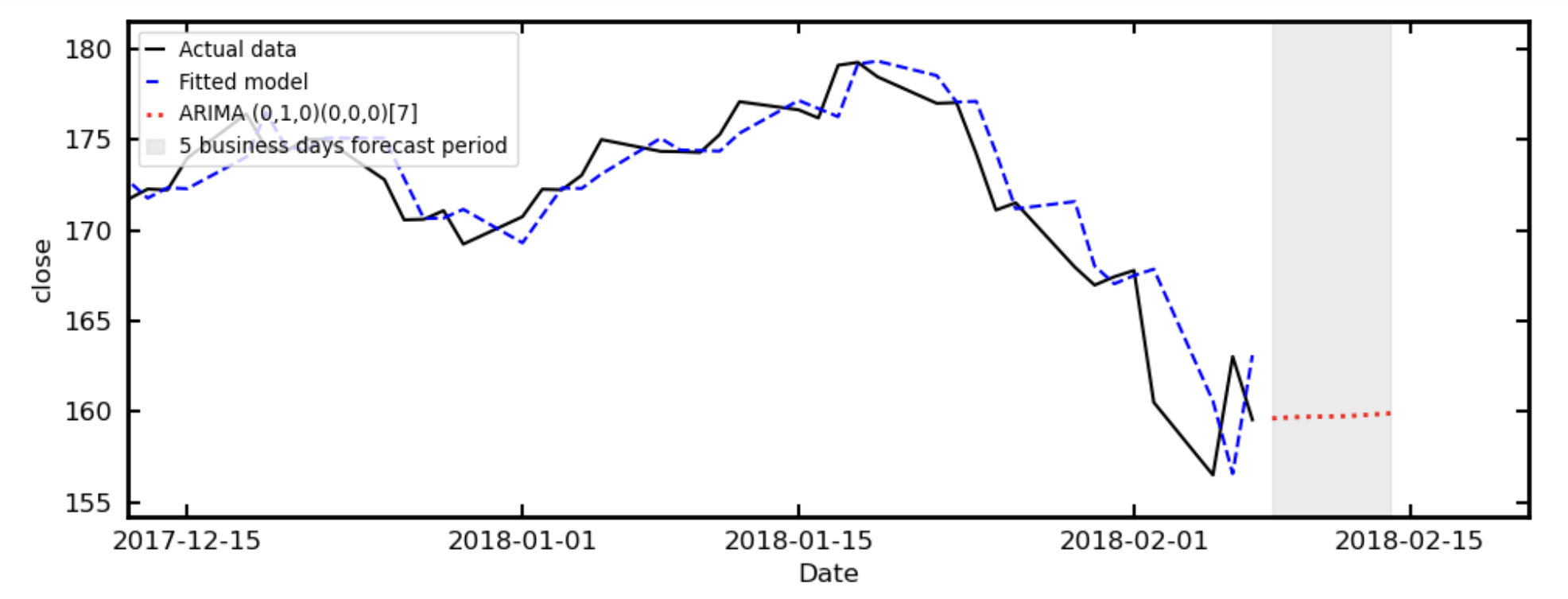
Which, like the simple exponential sample at Master Simple Exponential Smoothing for Time Series Forecasting, fails to accurately forecast the drop suffered by all companies over this period (driven by rising bond yields, fears on inflation and a crypto crash).

This demonstrates that even well-performing models can fail under changing conditions, reinforcing the importance of evaluating models beyond in-sample fit.